Scaling Nektar++ to 65K CPUs on ARCHER2
The recent capability day on ARCHER2 allowed us to study the performance of the IncNavierStokesSolver in Nektar++ up to 65536 CPUs. We will discuss the strong scaling of the solver using the current best-practise configuration for an aerodynamic test case inspired by the Formula 1 industry.
Best-practice for IncNavierStokesSolver
We are using the best-practise setup for IncNavierStokesSolver with the semi-implicit velocity correction scheme that is SolverType=VelocityCorrectionScheme with second order time-stepping. We additionally use the option SpectralHPDealiasing which enables dealiasing for the explicit advection operator, see the work by Mengaldo et al. (2023) for details. The setup for this study is available in the session file:
<CONDITIONS>
<SOLVERINFO>
    <I PROPERTY="SolverType"            VALUE="VelocityCorrectionScheme"/>
    <I PROPERTY="EQTYPE"                VALUE="UnsteadyNavierStokes"/>
    <I PROPERTY="EvolutionOperator"     VALUE="Nonlinear"/>
    <I PROPERTY="Projection"            VALUE="Continuous"/>
    <I PROPERTY="Driver"                VALUE="Standard"/>
    <I PROPERTY="SPECTRALHPDEALIASING"  VALUE="True"/>
    <I PROPERTY="SpectralVanishingViscosity" VALUE="DGKernel"/>
</SOLVERINFO>

<TIMEINTEGRATIONSCHEME>
    <METHOD> IMEX </METHOD>
    <ORDER> 2 </ORDER>
</TIMEINTEGRATIONSCHEME>
</CONDITIONS>
We achieve our current best performance with a matrix-based approach for solving the pressure and velocity problems. In particular, we employ static condensation with a Conjugate Gradient solver and use a Diagonal and LowEnergyBlock preconditioner for pressure and velocity, respectively. The stopping criteria is a tolerance based on the magnitude of the residual . This setup is configured within the GlobalSysSolnInfo block see the table and example session file below. Note that this setup is a slightly updated version from the previous blog post https://www.nektar.info/setting-up-industrial-simulations-using-incompressible-navier-stokes-solver/.
| Variable | GlobalSysSoln | Preconditioner | (Absolute)Tolerance |
|---|---|---|---|
| p | IterativeStaticCond | Diagonal | 1e-4 |
| u, v, w | IterativeStaticCond | LowEnergyBlock | 1e-2 |
<CONDITIONS>
<GLOBALSYSSOLNINFO>
    <V VAR="p">
        <I PROPERTY="GlobalSysSoln"             VALUE="IterativeStaticCond"/>
        <I PROPERTY="Preconditioner"            VALUE="Diagonal"/>
        <I PROPERTY="IterativeSolverTolerance"  VALUE="1e-4"/>
        <I PROPERTY="AbsoluteTolerance"         VALUE="True"/>
    </V>
    <V VAR="u,v,w">
        <I PROPERTY="GlobalSysSoln"             VALUE="IterativeStaticCond"/>
        <I PROPERTY="Preconditioner"            VALUE="LowEnergyBlock"/>
        <I PROPERTY="IterativeSolverTolerance"  VALUE="1e-2"/>
        <I PROPERTY="AbsoluteTolerance"         VALUE="True"/>
    </V>
</GLOBALSYSSOLNINFO>
</CONDITIONS>
ARCHER2 modules, compilation and slurm submission
We build Nektar++ v5.7 for this test following the guide in https://www.nektar.info/nektar-on-archer2-2/ however we enable advanced vector extension (AVX) for the compilation in order to improve the performance of compute-heavy operations. Note that ARCHER2’s CPUs are of type AMD EPYC 7742 and support AVX2, however, not AVX512, see https://docs.archer2.ac.uk/user-guide/hardware/ for details. The additional cmake argument to enable AVX2 is -DNEKTAR_ENABLE_SIMD_AVX2=ON.
The slurm submission differs from the Nektar++ guide above by using a few options specific to the ARCHER2 environment. Following the recommendations on https://docs.archer2.ac.uk/user-guide/scheduler/, we enforce interconnect locality with the option #SBATCH --switches=1 (or 2, 3, 4 depending on the number of nodes).
Nektar++ further supports the Hierarchical Data Format (HDF) version 5 for parallel reading and writing of the mesh, checkpoint files and other data. We use HDF5 with the incompressible flow solver through two additional command line arguments. First, the “–io-format=Hdf5” (or shortform “-i Hdf5”) argument enables parallel IO of files using HDF5. Second, we use “–use-hdf5-node-comm” to read meshes with a communicator per node instead of per MPI rank. This enables more efficient mesh reading when we use a large number of nodes in parallel. The final command in the slurm submission file is
srun IncNavierStokesSolver mesh.xml session.xml -i Hdf5 --use-hdf5-node-commThe Imperial Front Wing test case
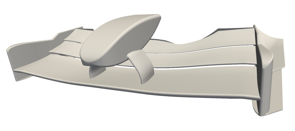
The test case is the Imperial Front Wing a multi-component wing in ground effect, see image below. We use an unstructured mesh composed of a total of 2.6 million mesh elements. The mesh is split into 1 million prismatic elements near any surfaces and 1.6 million tetrahedral elements to approximate the volume. The test case is characterised by a turbulent boundary layer flow across the wing components and a system of vortices forming from the wing. The flow around the wing has been studied previously in Pegrum (2006), Lombard (2017), Buscariolo (2022) and the geometry is openly available under this link https://doi.org/10.14469/hpc/6049.
Strong scaling study
We perform a strong scaling study using the mesh described above. We vary only the number of processors for the simulation and compare the average time per time step (excluding the initial setup time). We investigate the range from 2048 up to 65536 processors using fully populated nodes. Note that a node on ARCHER2 has 128 processors hence the study ranges from 16 to 512 nodes. Also, we use “CPU”, “processor” and “MPI rank” as synonyms in the following.
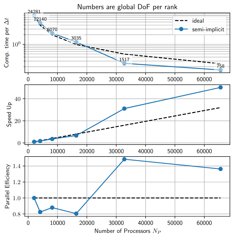
The strong scaling in Figure 1 shows that the incompressible Solver achieves a parallel efficiency of about 80% for processors. For larger number of cores, the parallel efficiency becomes larger than 1 which indicates that the performance is sub-optimal for processors. Considering the top plot, we see that the efficiency increases as we decrease the global degrees of freedom (DoF) per MPI rank from 3035 to 1517. This suggests a bottleneck in the memory bandwidth that is overcome as each rank holds fewer global DoFs and, hence, smaller matrices. The previous study by Lindblad et al. (2024) found a similar result for the compressible solver in Nektar++.
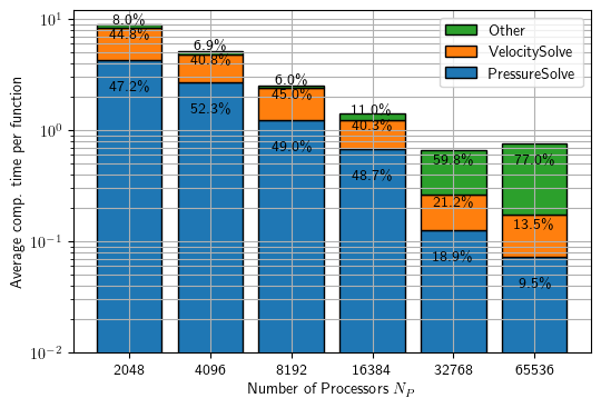
Figure 2 gives an overview of the contribution of critical functions with increasing number of processors. We find that for up to 16384 processors, the incompressible solver spends about 40% of the time per time step for solving the three Helmholtz problems, one for each velocity component, and another 45-50% for solving the pressure Poisson problem. The increase in “other” becomes significant for > 16384 processors and is mainly due to a large contribution of writing output files on this large-scale.
Lessons learned
In summary, the strong scaling study indicates a memory-bound performance for the matrix-based incompressible solver IncNavierStokesSolver within Nektar++. This motivates a matrix-free approach which consumes less memory by computing a matrix on the fly. Additionally, the study shows that parallel in-/output becomes a bottleneck at large scale.
We found, after completing this study, that we did not use the parallel file system Lustre efficiently on ARCHER2. As the ARCHER2 course on parallel IO explains here https://www.archer2.ac.uk/training/courses/251125-efficient-parallel-io/, one needs to manually set the stripe count on lustre such that the parallel filesystem is used effectively. This is possible by adding the following commands to the slurm submission script:
...
lfs setstripe -c -1 $SLURM_SUBMIT_DIR
lfs getstripe $SLURM_SUBMIT_DIR
...