Post-processing flow fields in the finite-difference grid
The visualisation of the flow fields output by Nektar++ looks not smooth if the resolution is not enough.
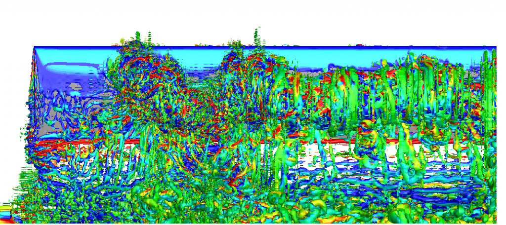
Figure 1 is an example of the leading-edge vortex generated by a plunging wing at Reynolds number 10,000. The result is from paper: Son, O., Gao, A., Gursul, I., Cantwell, C., Wang, Z., & Sherwin, S. (2022). Leading-edge vortex dynamics on plunging airfoils and wings. Journal of Fluid Mechanics, 940, A28. doi:10.1017/jfm.2022.224. Although there are 40M degrees of freedom for each velocity component, the discontinuities between element boundaries are still very obvious and the vortex looks not smooth.
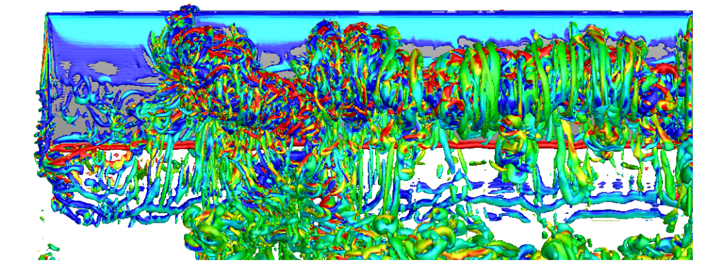
FieldConvert -m QCriterion -m vorticity)A feasible solution is interpolating the spectral element field to a finite difference grid and then doing the post-processing using the finite difference method. In figure 2, the spectral element field is first interpolated into 301 x 301 x 601 grid in the domain [-0.5, 2.5] x [-0.5, 1.5] x [0, 5.5]. Then the vorticity and Q are calculated using a second-order central difference scheme. The Q iso-surface looks much smoother.
The bash script to do the interpolation is
for((n=64; n<=64; n+=1))
do
mpirun -np 12 $NEKBIN/FieldConvert -f -e -v -m \
interppoints:fromxml=wing.xml:fromfld=wing_${n}.chk:box=301,301,601,-0.5,2.5,-0.5,1.5,0,5.5 \
interp${n}.plt
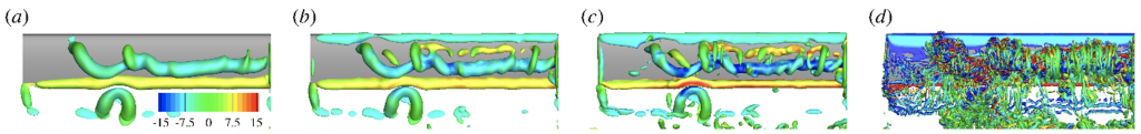
doneIn the finite-difference grid, a Gaussian filter can be easily applied by convolution operation to remove small scale vortices. Figure 3 shows that with decreasing filter size, there are more and more small scale vortices in the Q iso-surface.
The same operation can also be applied to 2D and 3DH1D fields. The finite different tool is a small c++ code available here https://github.com/gaoak/ptspostprocessing