There are various solvers built in Nektar++ that are designed with different features. Currently, there lacks a study that compares the computational resources (mainly run speed) between these solvers. Therefore, this article provides some results on the comparison of 4 different solver setups that are commonly used based on 2 standard benchmark cases. The idea is to run the solvers in the way that a typical user would. Meantime, the fastest configuration for each solver is explored by adjusting common parameters.

Solvers being compared:

• Incompressible Quasi-3D
• Incompressible 3D
• Explicit Compressible
• Implicit Compressible

Test cases used:

• Taylor – Green Vortex
• Turbulent Flow over Cylinder

Solver set-up

For each solver, the general parameters are set to typical values. The time step size used has been tested to be the largest/fastest possible. All the solvers uses the same number of quadrature points. In the case of the quasi-3D setup, the number of Fourier planes in the homogenous dimension is chosen to be the same as that of free quadrature points in the spectral/hp dimensions. Preconditioners are applied to the incompressible 3D setup as they usually are to improve performance. When performing the speed evaluation, all the filters and check files are disabled. They are output by doing another run in order to validate the results obtained.

Taylor – Green vortex

The Taylor – Green Vortex is a case with simple geometry but complicate turbulent flow mechanisms. Thus it provides a non-trivial case to solve but easy to set up and visualise/compare the results. Details can be found in the tutorial page. The results in this section are all obtained with polynomial order 4 (NUMMODE=5).

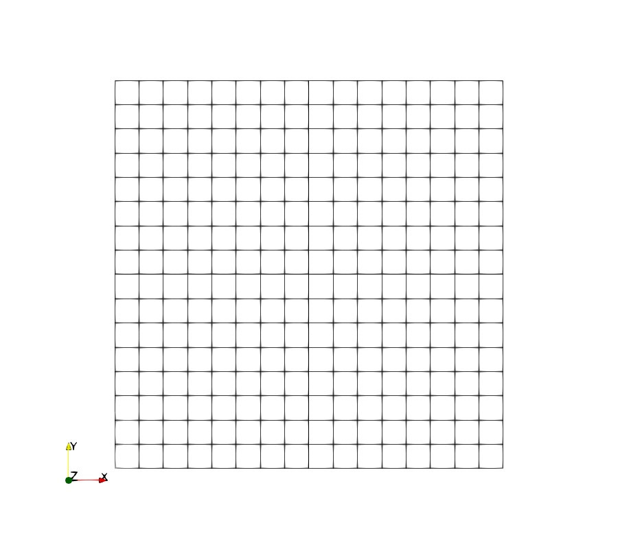
Mesh

The 3D Taylor – Green Vortex (TGV) uses a cubic mesh. In this study, the mesh size is 2pi x 2pi x 2pi and contains 4096 elements (16 x 16 x 16). For the quasi-3D setup, the 2D mesh is simply a extracted plane of the 3D mesh.

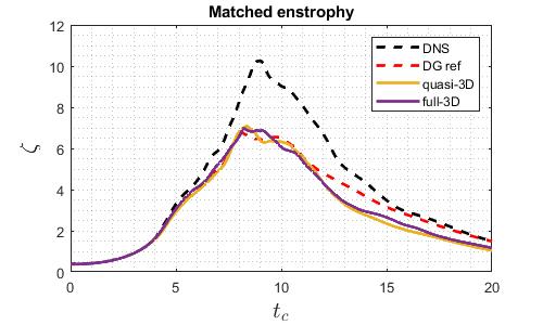
SVV coefficient

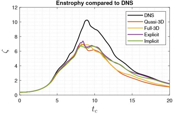
To achieve a good match of enstrophy of the DG kernel and the discontinuous Galerkin solvers. The DG SVVDiffCoeff is reduced from 1 to 0.0125. In the spectral dimension of quasi-3D solver, the exponential SVV kernel has SVVCutoffRatio=0.5, SVVDiffCoeff=0.1. The resulting enstrophy is shown below.

Time step study

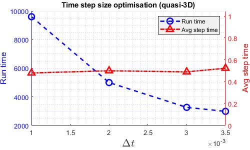
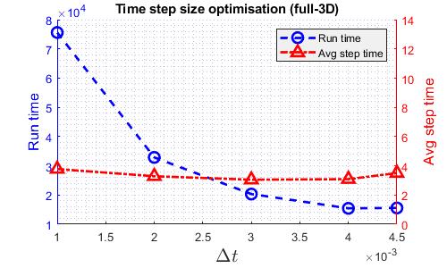
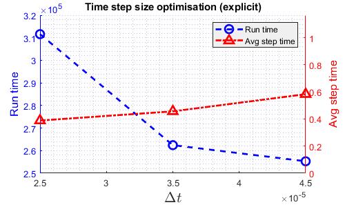
The aim for the timestep study is to identify the largest timestep that the solvers are able to run at so that each solver is running at the fastest speed. for efficiency, here, the results are obtained using more number of cores than the actual comparison run. However, the results should still apply. The following graphs shows how the run time varies with time step size for various solvers. “Avg Step Time” indicates the average time taken to solve one timestep. This has an impact on whether and how much does run time reduces as time step size increases. The largest time steps in these plots are the largest time step the solver can run through.

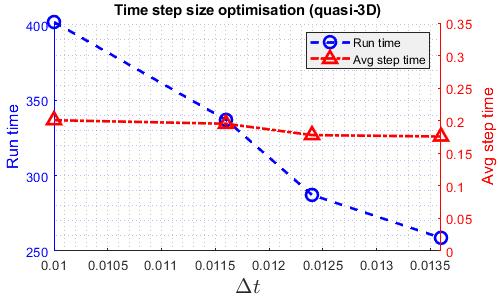
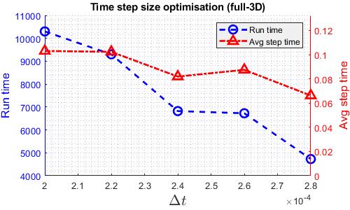
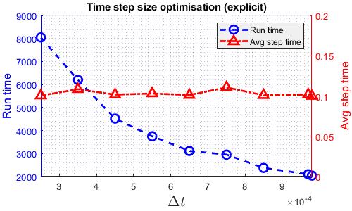
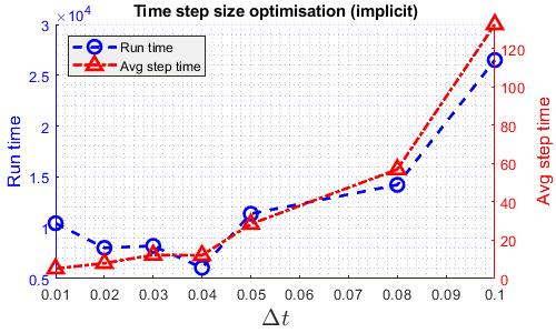
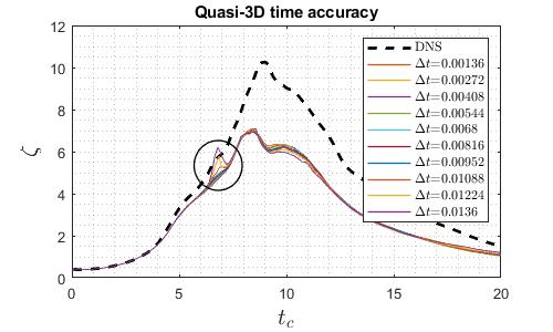
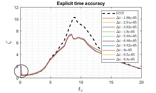
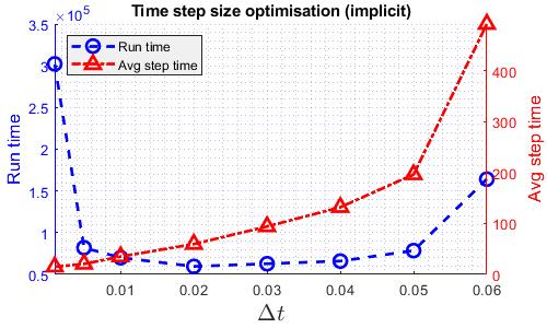
As shown in the graphs, for quasi-3D, 3D and explicit compressible solvers, the relation between runtime and time step size is almost linear as the average step time is roughly constant. However, for the implicit compressible solver, there is a minimum runtime. This is due to the Newton iterative solver built in the implicit Runge-Kutta scheme. As time step size increases, it takes more iteration to converge, hence the increasing average step time. The temporal accuracy is then checked, the time step size of quasi-3D and explicit solver is reduced to eliminate significant temporal error as shown below.

The final optimum time step size for each solver is summarised below.

Solvers	Quasi-3D	Full-3D	Explicit	Implicit
Time step size	0.0095	0.00028	0.0009	0.040

Speed comparison

The speed comparison between solvers are then performed. All runs are performed on the CX1 cluster under “single node” class (24 CPUs of model Intel(R) Xeon(R) CPU E5-2650 v4 @ 2.20GHz). The results is illustrated by the graph below. The average step time and time step size are normalised (divided) by that of the quasi-3D setup.

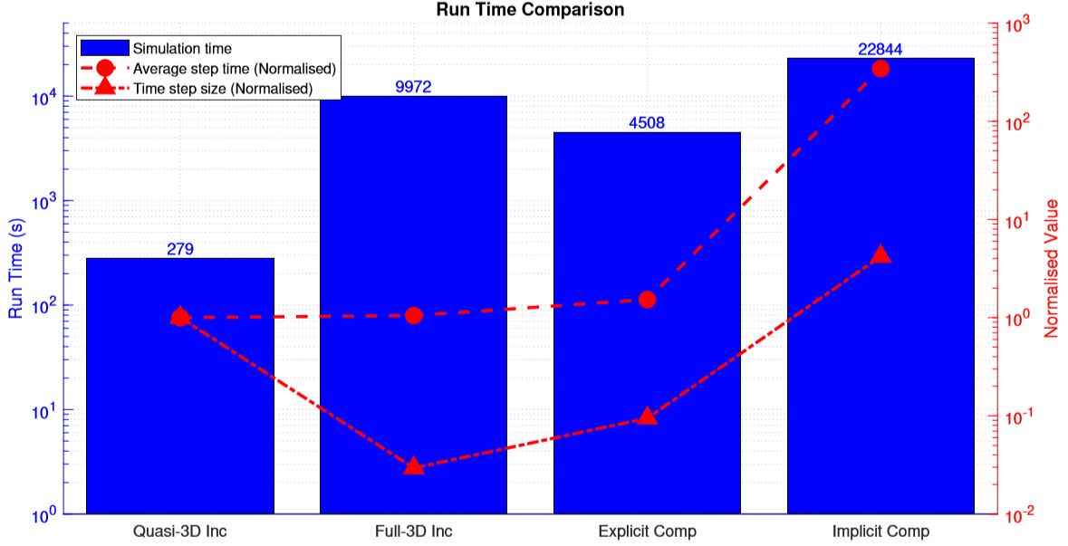
The quasi-3D set up is orders of magnitude faster than the others. The incompressible 3D solver is inefficient due to the much smaller time step required. The explicit compressible solver is over performing at test case by allowing a unusually large time step. As a result, the performance of the implicit compressible solver looks much worse. The higher than usual polynomial order used also contributes to the bad performance of the implicit solver.

Results validation

The enstrophy plots of the four setups are shown below for a quick results validation.

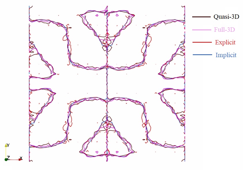
The contour of u=0 at periodic plane z is plotted for comparison.

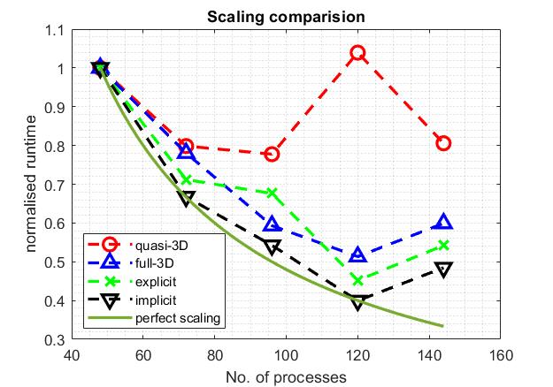
Scaling

A strong scaling test has been done under the “large” class. The number of processes increases from 48 (2 nodes) to 144 (6 nodes). Due to the small problem size, the quasi-3D hardly shows any scaling with more than 72 processes. The compressible solvers scales better than the incompressible ones. This is likely due to worse scalability of the global matrix operations.

Polynomial order study

In order to illustrate how does solver speed varies with order of accuracy, the run time for all the solvers at polynomial order 2 to 6 are plotted below. It can be seen that the implicit solver run-time increases at the highest exponential rate with polynomial order. The log slope of the other 3 solvers is similar.

Flow over cylinder

The flow over cylinder case is larger compare to the TGV. It resembles, to a greater extent, an actual case people would simulate. The more complicated mesh and flow features provide a more complete picture of the performance of various solvers. The results in this section is obtained with polynomial order 2 (NUMMODE=3).

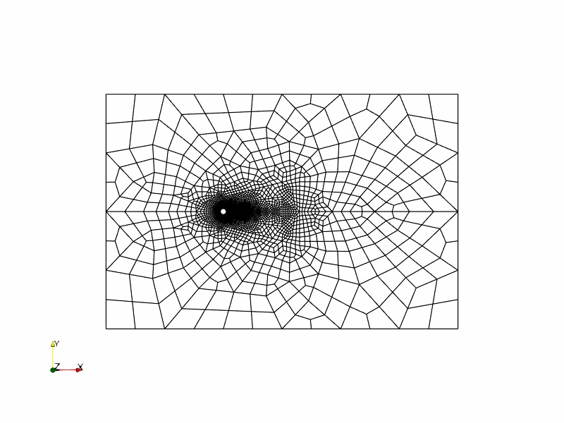
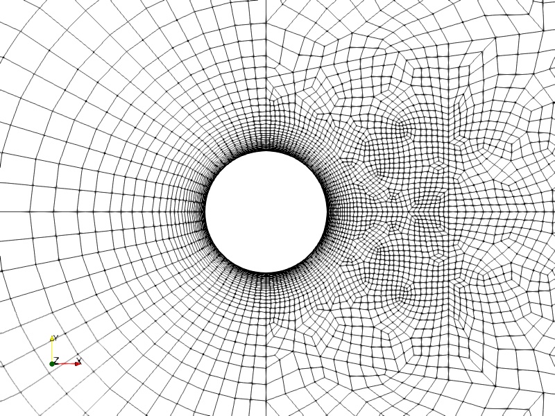
Mesh

The mesh used for this study is a all quad mesh in 2D and extruded by pi to obtain the 3D mesh. The mesh and detail view of the curved cylinder surface is shown below.

Time step study

Similar to the TGV case, finding the fastest time step size gives a more fair comparison among the solvers. The following graphs shows how runtime varies with time step size for various solvers. Note that the DG kernel coefficient used for the cylinder case is the standard value of 1.

The time step size used for speed comparison are listed in the table below.

Solvers	Quasi-3D	3D	Explicit	Implicit
Time step size	0.0035	0.0045	0.000045	0.020

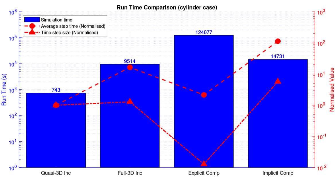
Speed comparison

The speed comparison are performed with 240 cores under the “large” class on CX1 (10 nodes of 24 CPU of model Intel(R) Xeon(R) CPU E5-2680 v3 @ 2.50GHz). The runtime comparison are shown in the graph below. With extensive grid stretching, the explicit solver suffers a much worse stability resulting in extremely small time step sizes and the longest run time. The stability of implicit solver is much less impacted and shows its speed advantage. Also, removing the triply periodic boundary condition seems to improve the stability of full-3D solver significantly allowing it to have similar time step size as the quasi-3D solver.

Results validation

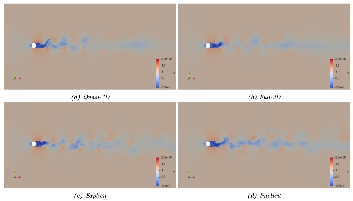
The post transient wake structure of the four solvers are similar as shown below.

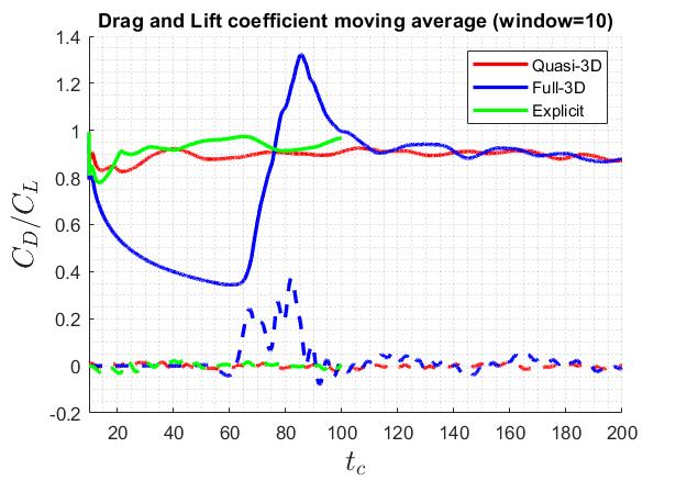
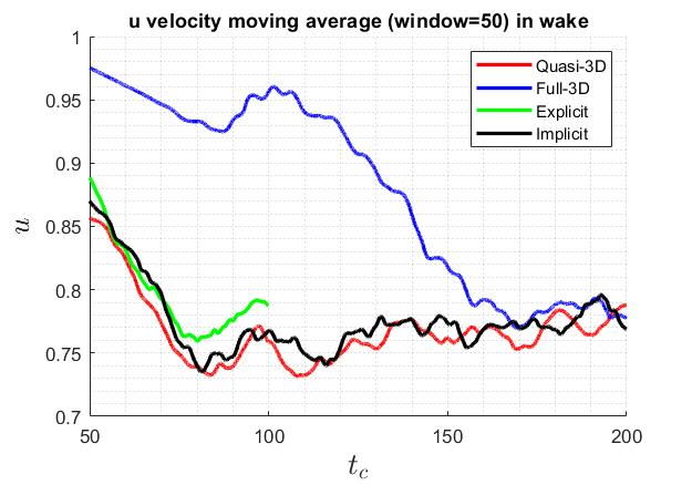
The lift and drag coefficient converges towards the same level as shown below. The “aeroforces” filter gives erroneous results for the implicit solver. Thus, the u velocity at a history point 15 diameter downstream are plotted as well. Explicit solver only has results up to t=100 due to long run-time.

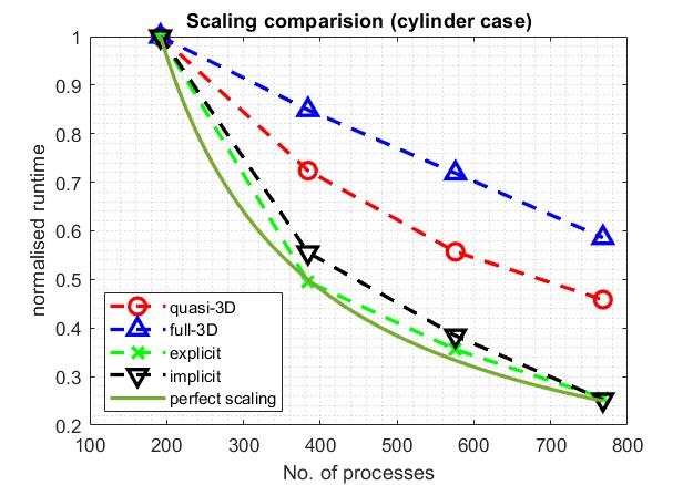
Scaling

Similar to the TGV case, a strong scaling test is performed on the cylinder case. Again, the compressible (DG) solvers are more scalable than the incompressible (CG) solvers. The full-3D solver is the least scalable which is likely caused by the preconditioners used in the iterative solver.

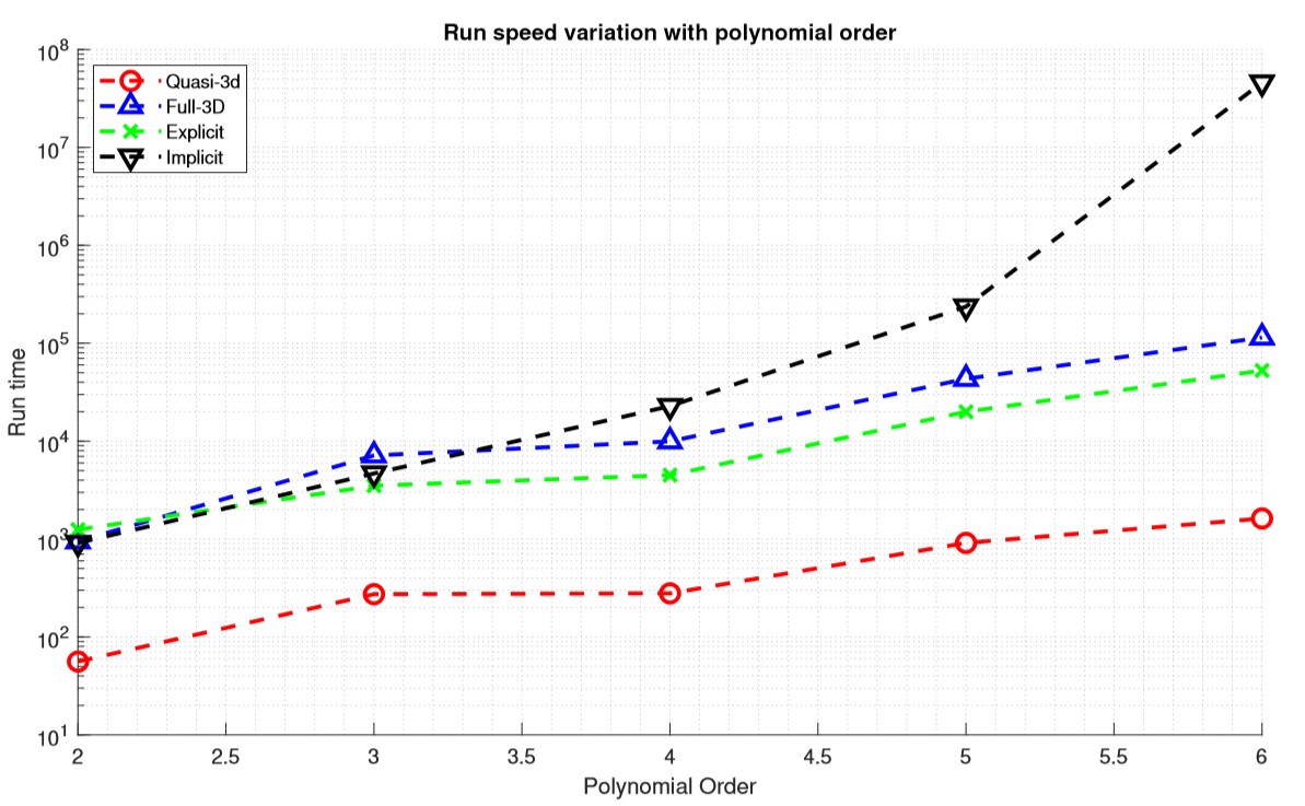
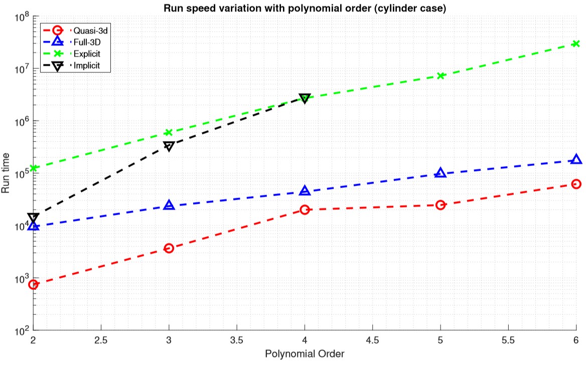
Polynomial order study

The run speed of four solvers for 2nd to 6th polynomial order are plotted for the cylinder case as well. The implicit solver is only tested up to 4th order due to RAM limit. Similar to the TGV case, the implicit solver has the fastest increase run-time with polynomial order. However, in the cylinder case, the full-3D solver clearly has the shallowest slope.

Files

The session and mesh files used for the speed comparison can be found at: https://www.nektar.info/wp-content/uploads/2020/06/comparison-files.zip