Compressible flow solver: Basics of the explicit solver
Prerequisite
- For this tutorial it is assumed that you are already familiar with the methods to non-dimensionalize the compressible flow you are interested in, and the paameters needed for the Nektar++ session file. If you need to review the non-dimensionalization see the tutorial
Compressible flow solver: Non-dimensionalizationfirst.
Learning objectives
Upon completion of this tutorial, the user will be able to
-
Get to know the session file parameters for the explicit compressible flow solver
-
Simulate the flow over a cylinder
- 1. Introduction
- 2. Session file
- 3. Expansions
- 4. Conditions
- 5. Run the solver
- 6. Visualisation in vtk.js
1. Introduction
Continued from the previous tutorial about no-dimensionalization, following which we can obtain the normalized flow parameters, in this tutorial we are going to complete the session file for a compressible flow case using the explicit solver. (The settings for the implicit solver will be introduced in the following tutorial.) A 2D compressible cylinder flow case is employed for the clearity of demonstration. The sketch of the geometry and settings are as follows.
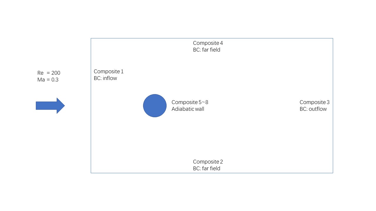 |
| Figure: Computational Domain |
2. Session file
| Top | Prev | Next |
The session file has .xml (Extensible Markup Language) extension, which allows the file to be organized in building blocks, and that all the settings and mesh can be in a single file or multiple ones. In many cases, as well as the one used in this tutorial, the parameters defining the flow conditions and controlling the solver are placed in the session.xml while the mesh is put in a seperate file named after the geometry, e.g. cylinder2D.xml. The benefit for doing so is to avoid opening the mesh file (often in binary) while modifying the settings, which is friendlier for some text editors.
Note If the mesh is in mesh.xml and the other settings are in session.xml, the mesh.xml needs to be entered before the session,xml when you call the solver. For example
CompressibleFlowSolver mesh.xml session.xml
3. Expansions
| Top | Prev | Next |
The first section to be set is the expansions. It defines the polynomial expansions used on each of the defined geometric composites. Expansion entries specify the number of modes, the basis type. The short-hand version has the following form
    <EXPANSIONS>
      <E COMPOSITE="C[100,101]" NUMMODES="3" FIELDS="rho,rhou,rhov,E" TYPE="MODIFIED" />
    </EXPANSIONS>
Here, the setting is initiated with E for expansion, the capital C is the initial for Composite. In the current version of Nektar++, the numbering for mesh composite starts from 100. As we use hybrid mesh generated by NekMesh, where triangular mesh is generated first and quadrilateral boundary layer mesh is then generated, C[100] and C[101] represent the triangluar mesh and quadrilateral mesh, respectly. The NUMMODES is the number of modes for polynomial expansions. This number equals to the order of polynomials plus one as the order of trial functions starts from zero. Considering the cost for this tutorial, we use 3 for NUMMODES, which can be increased to 5 for better resolution. As for the FIELDS, the four conservative variables for the 2D compressible flow are solved. The MODIFIED in the end adopts the default settings for quadrature points and etc.
4. Conditions
| Top | Prev | Next |
The conditions section contains the parameters to define the flow condition and set up the solver. The following five sub-sections are included.
4.1. Solver information
The solver information sets up the numerical methods employed in the session. Here is an example for the completed section.
    <SOLVERINFO>
      <I PROPERTY="EQType"                VALUE="NavierStokesCFE"     />
      <I PROPERTY="Projection"            VALUE="DisContinuous"       />
      <I PROPERTY="AdvectionType"         VALUE="WeakDG"              />
      <I PROPERTY="DiffusionType"         VALUE="LDGNS"               />
      <I PROPERTY="TimeIntegrationMethod" VALUE="ForwardEuler"        />
      <I PROPERTY="UpwindType"            VALUE="HLLC"                />
      <I PROPERTY="ProblemType"           VALUE="General"             />
      <I PROPERTY="EquationOfState"       VALUE="IdealGas"            />
      <I PROPERTY="ViscosityType"         VALUE="Variable"            />
    </SOLVERINFO>
-
EQTypeis the tag which specify the equations we want solve; -
Projectionis the type of projection we want to use; -
AdvectionTypeis the advection operator we want to use; -
DiffusionTypeis the diffusion operator we want to use for the Navier-Stokes equations; -
TimeIntegrationMethodis the time-integration scheme we want to use. Note that only an explicit discretisation is supported; -
UpwindTypeis the numerical interface flux (i.e. Riemann solver) we want to use for the advection operator; -
EquationOfStateallows selecting an equation of state for accounting for non-ideal gas behaviour; -
ViscosityTypeis the viscosity type we want to use.
Note The available options for above properties can be found in the User Guide.
4.2. Parameters
We list all the parameters under this section. Some parameters, such as TimeStep and NumSteps are necessary for the solver while the users are also free to define other parameters for the convenience of later usage. A completed parameters section will be as follows:
    <PARAMETERS>
      <P> TimeStep            = 0.0033                          </P>
      <P> NumSteps            = 7500                            </P>
      <P> IO_CheckSteps       = 2500                            </P>
      <P> IO_InfoSteps        = 200                             </P>
      <P> IO_CFLSteps         = 200                             </P>
      <P> Gamma               = 1.4                             </P>
      <P> Pr                  = 0.72                            </P>
      <P> Mach                = 0.3                             </P>
      <P> Re                  = 200.0                           </P>
      <P> GasConstant         = 1.0/(Gamma*Mach*Mach)           </P>
      <P> mu                  = 1.0/Re                          </P>
      <P> Tref                = 293.15                          </P>
      <P> rhoInf              = 1.0                             </P>
      <P> TInf                = 1.0                             </P>
      <P> pInf                = rhoInf*GasConstant*TInf         </P>
      <P> cInf                = sqrt(Gamma*GasConstant*TInf)    </P>
      <P> uInf                = Mach*cInf                       </P>
      <P> vInf                = 0.0                             </P>
      <P> wInf                = 0.0                             </P>
    </PARAMETERS>
-
TimeStepis the time-step we want to use; -
FinTimeis the final physical time at which we want our simulation to stop; -
NumStepsis the equivalent of FinTime but instead of specifying the physical final time we specify the number of time-steps; -
IO_CheckStepssets the number of steps between successive checkpoint files; -
IO_InfoStepssets the number of steps between successive info stats are printed to screen; -
Gammaratio of the specific heats. Default value = 1.4; -
PrPrandtl number. Default value = 0.72; -
MaMach number -
ReReynolds number -
GasConstantgas constant -
mureference dynamic viscosity (i.e. $\mu_{\infty}$). $\mu = Const$ or $\mu=\mu(T_{ref})$. Default value = 1.78e-05 Pas; -
Trefreference temperature (i.e. $T_{ref}$) at which the dynamic density is computed whenViscosityTypeis set to beVariable. The computation should follow the Sutherland’s law. Its value should be always in Kelvin. -
rhoInffarfield density (i.e. $\rho_{\infty}$). Default value = 1.225 Kg/m3; -
TInffarfield temperature (i.e. $T_{\infty}$). Default value = 288.15 K; -
pInffarfield pressure (i.e. $p_{\infty}$). Default value = 101325 Pa; -
Twalltemperature at the wall when isothermal boundary conditions are employed (i.e. $T_{wall}$). Default value = 300.15K; -
uInffarfield X-component of the velocity (i.e. $u_{\infty}$). Default value = 0.1 m/s; -
vInffarfield Y -component of the velocity (i.e. $v_{\infty}$). Default value = 0.0 m/s; -
wInffarfield Z-component of the velocity (i.e. $w_{\infty}$). Default value = 0.0 m/s;
Note that users can define their own parameters which can be used in the session file for expression simpility (i.e. Ma and Re in the above list.)
4.3. Variables
Similar to the expansions, the four conservative variables need to be typed under the variables tag
    <VARIABLES>
      <V ID="0"> rho  </V>
      <V ID="1"> rhou </V>
      <V ID="2"> rhov </V>
      <V ID="3"> E    </V>
    </VARIABLES>
4.4. Boundary regions and conditions
After having defined the variables depending on the dimensions of the problem we want to solve, it is necessary to specify the boundary regions on which we want to define the boundary conditions. According to the sketch, composites 5~8 represent the adiabatic wall, composite 1 represents the inflow boundary, composite 2 and 4 represent the far field boundary, composite 4 represents the outflow boundary. For simplicity, far field boundary condition is applied to all the boundaries except the wall.
    <BOUNDARYREGIONS>
      <!-- 1-inflow (left), 2-Farfield (bottom), 3-Outflow (right)
           4-Farfield (top), 5,6,7,8-Wall (cylinder) -->
      <B ID="0"> C[5-8] </B>    <!-- Wall      -->
      <B ID="1"> C[1]   </B>    <!-- Inflow    -->
      <B ID="2"> C[3]   </B>    <!-- Outflow   -->
      <B ID="3"> C[2,4] </B>    <!-- Farfield -->
    </BOUNDARYREGIONS>

    <BOUNDARYCONDITIONS>
      <!-- Wall -->
      <REGION REF="0">
        <D VAR="rho"  USERDEFINEDTYPE="WallAdiabatic" VALUE="0" />
        <D VAR="rhou" USERDEFINEDTYPE="WallAdiabatic" VALUE="0" />
        <D VAR="rhov" USERDEFINEDTYPE="WallAdiabatic" VALUE="0" />
        <D VAR="E"    USERDEFINEDTYPE="WallAdiabatic" VALUE="0" />
      </REGION>
      <!-- Inflow -->
      <REGION REF="1">
        <D VAR="rho"  VALUE="rhoInf"      />
        <D VAR="rhou" VALUE="rhoInf*uInf" />
        <D VAR="rhov" VALUE="rhoInf*vInf" />
        <D VAR="E"    VALUE="pInf/(Gamma-1) + 0.5*rhoInf*(uInf*uInf + vInf*vInf)" />
      </REGION>
      <!-- Outflow -->
      <REGION REF="2">
        <D VAR="rho"  VALUE="rhoInf"      />
        <D VAR="rhou" VALUE="rhoInf*uInf" />
        <D VAR="rhov" VALUE="rhoInf*vInf" />
        <D VAR="E"    VALUE="pInf/(Gamma-1) + 0.5*rhoInf*(uInf*uInf + vInf*vInf)" />
      </REGION>
      <!-- Farfield -->
      <REGION REF="3">
        <D VAR="rho"  VALUE="rhoInf"      />
        <D VAR="rhou" VALUE="rhoInf*uInf" />
        <D VAR="rhov" VALUE="rhoInf*vInf" />
        <D VAR="E"    VALUE="pInf/(Gamma-1) + 0.5*rhoInf*(uInf*uInf + vInf*vInf)" />
      </REGION>
    </BOUNDARYCONDITIONS>
4.5. Functions
The FUNCTIONin this session file is used to set initial condition. Otherwise all fields will be set to be zero for by default, which will cause NaN in the compressible flow simulations as the density and pressure must be positive in any time step.
    <FUNCTION NAME="InitialConditions">
      <E VAR="rho"  VALUE="rhoInf" />
      <E VAR="rhou" VALUE="rhoInf * uInf" />
      <E VAR="rhov" VALUE="rhoInf * vInf" />
      <E VAR="E"    VALUE="pInf / (Gamma - 1) + 0.5 * rhoInf * (uInf * uInf + vInf * vInf)" />
    </FUNCTION>
In other cases where exact solutions exist. ExactSolution can be applied to compute them. The exact solutions can then used as the references to evaluate the numerical solutions.
    <FUNCTION NAME="ExactSolution">
      <E VAR="rho"  VALUE="rhoInf" />
      <E VAR="rhou" VALUE="rhoInf*uInf" />
      <E VAR="rhov" VALUE="rhoInf*vInf" />
      <E VAR="E"    VALUE="pInf / (Gamma - 1) + 0.5 * rhoInf * (uInf * uInf + vInf * vInf + wInf * wInf)"/>
    </FUNCTION>
5. Running the solver
| Top | Prev | Next |
The following command is entered to run the compressible flow solver
CompressibleFlowSolver mesh.xml session.xml
The solver can be run in parallel using MPI
mpirun -np 8 CompressibleFlowSolver mesh.xml session.xml
However, as the Binder environment does not support MPI, this tutorial only run the solver in serial.
!CompressibleFlowSolver cyl2D.xml session.xml
=======================================================================
	        EquationType: NavierStokesCFE
	        Session Name: cyl2D
	        Spatial Dim.: 2
	  Max SEM Exp. Order: 3
	      Expansion Dim.: 2
	      Riemann Solver: HLLC
	      Advection Type:
	     Projection Type: Discontinuous Galerkin
	      Diffusion Type:
	           Advection: explicit
	       AdvectionType: WeakDG
	           Diffusion: explicit
	           Time Step: 0.0033
	        No. of Steps: 7500
	 Checkpoints (steps): 3000
	    Integration Type: ForwardEuler
=======================================================================
Initial Conditions:
  - Field rho: rhoInf
  - Field rhou: rhoInf*uInf
  - Field rhov: rhoInf*vInf
  - Field E: pInf/(Gamma-1) + 0.5*rhoInf*(uInf*uInf + vInf*vInf)
Writing: "cyl2D_0.chk" (0.00868509s, XML)
Steps: 200      Time: 0.66         CPU Time: 1.90324s
CFL: 0.320257 (in elmt 649)
Steps: 400      Time: 1.32         CPU Time: 1.9112s
CFL: 0.317977 (in elmt 638)
Steps: 600      Time: 1.98         CPU Time: 1.90547s
CFL: 0.316242 (in elmt 638)
Steps: 800      Time: 2.64         CPU Time: 1.9007s
CFL: 0.314456 (in elmt 638)
Steps: 1000     Time: 3.3          CPU Time: 1.89966s
CFL: 0.313848 (in elmt 638)
Steps: 1200     Time: 3.96         CPU Time: 1.9058s
CFL: 0.313332 (in elmt 638)
Steps: 1400     Time: 4.62         CPU Time: 1.91103s
CFL: 0.312854 (in elmt 638)
Steps: 1600     Time: 5.28         CPU Time: 1.90367s
CFL: 0.312576 (in elmt 638)
Steps: 1800     Time: 5.94         CPU Time: 1.90334s
CFL: 0.31234 (in elmt 638)
Steps: 2000     Time: 6.6          CPU Time: 1.90171s
CFL: 0.312055 (in elmt 638)
Steps: 2200     Time: 7.26         CPU Time: 1.90231s
CFL: 0.311384 (in elmt 638)
Steps: 2400     Time: 7.92         CPU Time: 1.89879s
CFL: 0.311312 (in elmt 638)
Steps: 2600     Time: 8.58         CPU Time: 1.89549s
CFL: 0.311 (in elmt 638)
Steps: 2800     Time: 9.24         CPU Time: 1.9021s
CFL: 0.310917 (in elmt 638)
Steps: 3000     Time: 9.9          CPU Time: 1.90342s
CFL: 0.310835 (in elmt 638)
Writing: "cyl2D_1.chk" (0.0228159s, XML)
Steps: 3200     Time: 10.56        CPU Time: 1.90888s
CFL: 0.310854 (in elmt 638)
Steps: 3400     Time: 11.22        CPU Time: 1.90654s
CFL: 0.310935 (in elmt 638)
Steps: 3600     Time: 11.88        CPU Time: 1.90566s
CFL: 0.311003 (in elmt 638)
Steps: 3800     Time: 12.54        CPU Time: 1.90936s
CFL: 0.311011 (in elmt 638)
Steps: 4000     Time: 13.2         CPU Time: 1.90714s
CFL: 0.310921 (in elmt 638)
Steps: 4200     Time: 13.86        CPU Time: 1.9098s
CFL: 0.31072 (in elmt 638)
Steps: 4400     Time: 14.52        CPU Time: 1.91911s
CFL: 0.310427 (in elmt 638)
Steps: 4600     Time: 15.18        CPU Time: 1.90739s
CFL: 0.310085 (in elmt 638)
Steps: 4800     Time: 15.84        CPU Time: 1.90489s
CFL: 0.309796 (in elmt 638)
Steps: 5000     Time: 16.5         CPU Time: 1.91068s
CFL: 0.30966 (in elmt 638)
Steps: 5200     Time: 17.16        CPU Time: 1.91043s
CFL: 0.30976 (in elmt 638)
Steps: 5400     Time: 17.82        CPU Time: 1.91101s
CFL: 0.310115 (in elmt 638)
Steps: 5600     Time: 18.48        CPU Time: 1.90595s
CFL: 0.310677 (in elmt 638)
Steps: 5800     Time: 19.14        CPU Time: 1.90897s
CFL: 0.311308 (in elmt 638)
Steps: 6000     Time: 19.8         CPU Time: 1.90278s
CFL: 0.311835 (in elmt 638)
Writing: "cyl2D_2.chk" (0.0226407s, XML)
Steps: 6200     Time: 20.46        CPU Time: 1.9106s
CFL: 0.312097 (in elmt 638)
Steps: 6400     Time: 21.12        CPU Time: 1.90579s
CFL: 0.311958 (in elmt 638)
Steps: 6600     Time: 21.78        CPU Time: 1.90246s
CFL: 0.311453 (in elmt 638)
Steps: 6800     Time: 22.44        CPU Time: 1.90575s
CFL: 0.31104 (in elmt 638)
Steps: 7000     Time: 23.1         CPU Time: 1.91266s
CFL: 0.311354 (in elmt 638)
Steps: 7200     Time: 23.76        CPU Time: 1.90362s
CFL: 0.312481 (in elmt 638)
Steps: 7400     Time: 24.42        CPU Time: 1.9027s
CFL: 0.313847 (in elmt 638)
Time-integration  : 71.4737s
Writing: "cyl2D.fld" (0.022676s, XML)
-------------------------------------------
Total Computation Time = 74s
-------------------------------------------
L 2 error (variable rho) : 12.1546
L inf error (variable rho) : 1.05503
L 2 error (variable rhou) : 12.3101
L inf error (variable rhou) : 1.41509
L 2 error (variable rhov) : 2.47569
L inf error (variable rhov) : 0.87864
L 2 error (variable E) : 247.609
L inf error (variable E) : 21.3563
6. Visualisation in vtk.js
| Top | Prev |
The cells below show how visualisation of a VTU output file from FieldConvert can be viewed directly in the notebook. First, we post-process with FieldConvert to produce a .vtu file.
!FieldConvert -f cyl2D.xml session.xml cyl2D.fld cyl2D_P2.vtu
Writing: "cyl2D_P2.vtu"
Written file: cyl2D_P2.vtu
Now we can use PyVista, combined with itkwidgets to visualise this in-browser as follows:
import pyvista as pv

# First read the VTK file
mesh = pv.read('cyl2D_P2.vtu')

# Now create an itkwidget to visualise this in-browser.
pl = pv.PlotterITK()
pl.add_mesh(mesh, scalars=mesh['u'], smooth_shading=True)
pl.show(True)
Viewer(geometries=[{'vtkClass': 'vtkPolyData', 'points': {'vtkClass': 'vtkPoints', 'name': '_points', 'numberO…
Viewer(geometries=[{'vtkClass': 'vtkPolyData', 'points': {'vtkClass': 'vtkPoints', 'name': '_points', 'numberO…
Try it yourself
Task 1
In the above session file we use NUMMODES=3 for fast completion of the solving. It has been tested to successfully produce vortex shedding while the resolution is not good enough. Now we try to resolve more details by increasing the number of modes to 5 as NUMMODES=5. Before we launch the simulation, we need to adjust the time step to make sure the simulation is stable. Find out a stable time step and complete the simulation.
Note Using a higher order polynomial expansion will cost more resources. The simulation might be quite slow in the binder environment. So it’s better to complete this case (and following ones) on you own computer.
Task 2
Since we are using scaled geometry and flow parameters, we can easily set up a different case with a few modifications. Try to launch a simulation with $Re = 3000$ and $Ma = 0.5$ by setting <P> Mach = 0.5 </P> and <P> Re = 3000.0 </P> under the <PARAMETERS>tag.
Note The current time step is specifically adjusted to be as large as possible for fast completion in the example. After you change the flow conditions, this value might needs further adjustment.
Task 3
Continued from the square cylinder flow case in Task 3, we will re-run this case using the isothermal wall boundary condition instead of the adiabatic wall. Now need the following settings for boundary condition:
      <REGION REF="0">
        <D VAR="rho"  USERDEFINEDTYPE="WallViscous" VALUE="0" />
        <D VAR="rhou" USERDEFINEDTYPE="WallViscous" VALUE="0" />
        <D VAR="rhov" USERDEFINEDTYPE="WallViscous" VALUE="0" />
        <D VAR="E"    USERDEFINEDTYPE="WallViscous" VALUE="0" />
      </REGION>
Note When we are using the isothermal wall, Twall should be set otherwise the default dimensional value will be used, which, in general, is not the desired value.
Take-a-ways
It is worth keeping in mind the following points:
- The conservative variables $(\rho, \rho u, \rho v, \rho w, E)$ will be used in the compressible flow solver, in contrast to the primitive variables $(u, v, w, p)$ in the incompressible flow solver.
- The boundary condition type in the compressible flow solver is always Dirichlet boundary condition, denoted by
<D>$. - Different boundary conditions are applied through
USERDEFINEDTYPE. If it is not defined, the input values afterVALUEwill be used as ghost state values for the Riemann solver to construct the numerial flux through the boundary.
References:
- Nektar++: Spectral/hp Element Framework, Version 5.0.1, User guide, January, 2021.