Incompressible Flow Simulation
Learning objectives
Welcome to the tutorial on the incompressible flow simulation using the Nektar++ framework. This tutorial aims to show how to setup and run a simulation for incompressible flows using the Nektar++ IncNavierStokesSolver for the well-known problem of external flow over a cylinder.
After completetion of this tutorial you will be familiar with:
- Configuring a XML file suitable for incompressible Navier-Stokes in Nektar++.
- Simulating 2D and quasi-3D incompressible flows.
- Running the simulation in serial and parallel.
- Computing aerodynamic forces and modal energy as a function of time.
- Post-processing the results and converting the Nektar++ field outputs for visualization.
Introduction
In this tutorial we will walk through how to configure a session file to be able to solve incompressible Navier-Stokes equations using a simple flow example. We consider flow over a circular cylinder. At the beginning we consider a two-dimensional case. Upon completion of the 2D case, we extend the problem to a quasi-3D case. By quasi-3D, we mean that the 2D mesh will be extruded in the spanwise direction, with periodic boundary conditions applied in the spanwise direction.
Governing equation
The incompressible solver implemented in Nektar++ uses the convective form of the Navier-Stokes equations for viscous incompressible and Newtonian fluids, which can be written as:
\begin{equation} \frac{\partial \mathbf{V}}{\partial t}+ \mathbf{V} \cdot \nabla \mathbf{V}=-\nabla p + \nu \nabla ^{2} \mathbf{V} + \mathbf{f} \end{equation}
\begin{equation} \nabla \cdot \mathbf{V} =0 \end{equation}
where $\mathbf{V} = (u,v,w)$ is the velocity of the fluid in the $x$, $y$, and $z$ directions, respectively, $p$ is the specific pressure (including density), $\nu$ is the kinematic viscosity, and $\mathbf{f}$ is the forcing term.
Problem description: 2D case
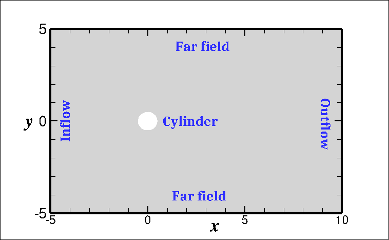
In this tutorial we use air to simulate the flow past a 2D circular cylinder with diameter $D=1$. For our study, we will use a Reynolds number $Re = 40$ with $Re = UD/\nu$ where $U$ is the velocity scale, $D$ is the length scale and $\nu$ is the kinematic viscosity.
The flow domain is a rectangle of sizes $[-5,10] \times [-5,5]$ as shown in the figure below.
 |
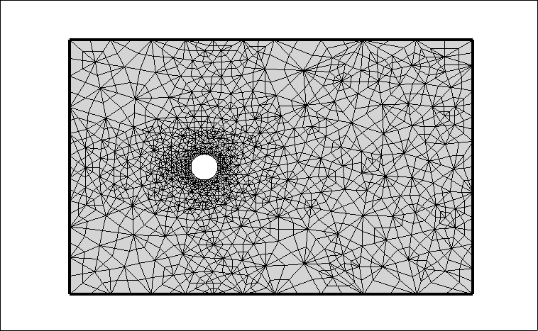 |
| Computational Domain | Computational Mesh |
We apply the following boundary conditions (BCs):
- no−slip conditions on the cylinder surface (i.e., homogeneous Dirichlet BC $\mathbf{V}=\mathbf{0}$);
- far−field with Dirichlet BC: $(u, v) = (1, 0)$ at the bottom and top boundaries;
- a corresonding inflow with Dirichlet BC: $(u, v) = (1, 0)$ at the left boundary;
- and an outflow at the right boundary with static pressure $p=0$.
Pre-processing
In this section we discuss how to setup the .xml files suitable for Nektar++ simulation. Here we use two separate XML files:
- A geometry XML file, which contains the mesh used to represent the computational domain;
- A session or conditions XML file, which contains simulation conditions, problem parameters, filters, etc.
Geometry tag from the geometry XML file into the session (condition) XML file to make a single XML file.
Please open the condition file session2d.xml. You will see three main tags (<EXPANSIONS>,<CONDITIONS> and <FILTERS>) within the <NEKTAR> tag as shown below:
<NEKTAR>
    <EXPANSIONS>
        <!-- The basis to be used in each element. -->
    </EXPANSIONS>
    <CONDITIONS>
        <!-- Solver-specific information, including boundary and initial conditions. -->
    </CONDITIONS>
    <FILTERS>
        <!-- Calculate a variety of quantities as the solution evolves in time. -->
    </FILTERS>
</NEKTAR>
Expansion bases
First, let us complete the <EXPANSIONS> tags.
Task 1:
Please write the missing parts in <EXPANSIONS> tag.
A completed <EXPANSIONS> tag has the following standard form:
 <EXPANSIONS>
        <E COMPOSITE="C[100,101]" NUMMODES="3" FIELDS="u,v,p" TYPE="MODIFIED" />
 </EXPANSIONS>`
Here,
COMPOSITErefers to the ID assigned to the geometric domain (or sub-domain) defined in the geometry xml file.NUMMODESis used to indentify the polynomial order of the expansion basis functions as $P = \texttt{NUMMODES}-1$.TYPEdenotes the basis functions. Possible choices areMODIFIED,GLL_LAGRANGE,GLL_LAGRANGE_SEM. One may note that the first basis type the modified modal expansion of Karniadakis & Sherwin, whereas the remaining two consider nodal expansion using Lagrange basis functions.
Conditions setup
Now, we will complete the <CONDITIONS> tag. There are five sections in this tag:
SOLVERINFOdefines solver setup (e.g. the equations to solve);PARAMETERSallow us to define solver parameters, such as $Re$ or the timestep size;VARIABLESdefine the scalar variables that will be solved for (i.e. $u$, $v$ and $p$);BOUNDARYREGIONSandBOUNDARYCONDITIONSdefine the boundary conditions;- finally we need a function to define the initial conditions for the problem.
Solver info
Task 2: Please complete the properties SolverType, EQTYPE, EvolutionOperator as shown below,
       <I PROPERTY="SolverType"           VALUE="VelocityCorrectionScheme"/>
       <I PROPERTY="EQTYPE"               VALUE="UnsteadyNavierStokes"    />
       <I PROPERTY="EvolutionOperator"    VALUE="Nonlinear"               />
Here,
SolverTypesets the algorithm we want to use to solve the governing equations.EQTYPEsets the kind of equations we want to solve. Here we useUnsteadyNavierStokessince we want to solve an unsteady-in-time Navier-Stokes solver; other options might be e.g.UnsteadyStokes, but this is not suitable for our problem.EvolutionOperatorsets the choice of the convection operator (i.e. the term $\mathbf{V}\cdot\nabla\mathbf{V}$):Nonlinearfor standard non-linear Navier-Stokes equationsDirectfor linearised Navier-Stokes equationsAdjointfor adjoint Navier-Stokes equationsTransientGrowthfor transient growth analysisSkewSymmetricfor skew symmetric form of the Navier-Stokes equations.
Parameters
In <PARAMETERS> tag, we can define the parameters present in the flow problem as well as the parameters required by various solvers of Nektar++. Hence a parameter can either be defined in the context of the problem we are solving (a ‘dummy’ or utility variable), or be predefined within Nektar++ (solver parameter). One should note that the names of the solver parameters can’t be altered, and some solvers will expect certain parameters to be defined.
Task 3: Assign values to the following parameters as
	      <P> TimeStep       = 0.025               </P>
          <P> FinTime        = 20.0                </P>
          <P> IO_CheckSteps  = NumSteps/20         </P>
          <P> Re             = 40                  </P>
Here,
TimeStepsets the time-step size for the time integration. One should select magnitude ofTimeStepstrategically to avoid the situation of CFL (Courant-Friedrichs-Lewy) number to be too large!FinTimeis used for define the final time of the simulation. Equivalently, one could specifyNumStepsto set the number of time-steps for the simulation. Given two ofTimeStep,FinTimeandNumSteps, Nektar++ will calculate the remaining quantity automatically.IO_CheckStepssets the number of steps between successive checkpoint files (which are saved as files ending in the extension.chk) to save the solution at equal-interval intermediate time levels. For example, sinceTimeStepis0.025andFinTimeis20.0, we have thatNumStepsis800. SinceIO_CheckStepsis then set asNumSteps/20which will generate twenty successive checkpoint files.Redenotes the Reynolds number used for the simulation. This is not explicitly required by the solver, i.e. it is a ‘dummy’ parameter.Kinvisdenotes kinematic viscosity of the fluid used and is required as a solver parameter. One may directly supply the value ofKinviswithout definingRein the XML file, but generally it is more convenient to adjust $Re$ as the quantity of interest.
Variables
In <VARIABLES> tag, we define the number (and name) of solution variables. We prescribed a unique ID to each variable.
Task 4: Provide a ID for the v-velocity component as
<V ID="1">v</V>
Boundary conditions
Boundary conditions are defined by two tags. First we define the boundary regions in the <BOUNDARYREGIONS> tag in terms of composite C[ ] entities from the <GEOMETRY> tag section of the mesh xml file. Each boundary region has a unique ID. For the current computational domain there are eight composites (see towards the bottom section of mesh xml file) marked as C[1] to C[8].
Task 5: Define the farfield region using C[2] and C[4] as shown below
<B ID="3"> C[2,4] </B> <!-- farfield -->
The next tag we define is <BOUNDARYCONDITIONS> tag, in which specify the boundary conditions for each boundary ID specified in the above <BOUNDARYREGIONS> tag.
Task 6: Define $u=1$, $v=0$ and higher-order pressure boundary condition for the inflow section as
            <REGION REF="1"> <!-- inflow   -->
                <D VAR="u" VALUE="1" />
                <D VAR="v" VALUE="0" />
                <N VAR="p" VALUE="0" USERDEFINEDTYPE="H" />
            </REGION>
Note the use of USERDEFINEDTYPE="H", which tells the IncNavierStokesSolver to set the high-order pressure boundary condition for $p$. In this case the VALUE attribute is ignored.
Initial conditions
Task 7: Provide the initial conditions $u(t=0)=1$, $v(t=0)=0$ and $p(t=0)=0$ in the “InitialConditions” FUNCTION as,
                 <E VAR="u" VALUE="1" />
                 <E VAR="v" VALUE="0" />
                 <E VAR="p" VALUE="0" />
Special parameters for solution stabilisation
One of the main challenges of running fluid simulations at high-order is numerical stability, since the low dissipation and diffusion at high orders can lead to accumulation of numerical errors in the presence of only mild under-resolution. The mesh we will use today is deliberably under-resolved to make it cheap to simulate. For this reason, we need to now enable some parameters in the <SOLVERINFO> tag to allow for the stabilisation of the incompressible flow solver.
Spectral vanishing viscosity
<I PROPERTY="SpectralVanishingViscosity" VALUE="DGKernel" />
-
SpectralVanishingViscosityactivates a stabilization technique that increases the viscosity on the modes with the highest frequencies. Possible options availabe areTrue,ExpKernel,DGKernelfor exponential, power and DG Kernel, respectively. -
To override the default values, we define the parameters
SVVCutoffRatioin the<PARAMETERS>tag as<P> SVVCutoffRatio = 0.5 </P>
To explore more about spectral vanishing viscoity one may consult with Ref. [2] and Section 11.3.1 of Ref. [1].
Spectral dealiasing
<I PROPERTY="SPECTRALHPDEALIASING" VALUE="True" />
SPECTRALHPDEALIASINGactivates the dealiasing (or over-integration) to stabilize the simulation. This dealiasing technique helps to reduce the numerical instability associated with the integration of the nonlinear terms [3]. One may note that Nektar++ also uses another dealiasing which is associated with the Fourier expansion considered in quasi-3D simulations and activates using the propertyDEALIASING.
Filter setup
<FILTER> tags are used for calculating a variety of useful quantities from the field variables as the solution evolves in time. There are several filters predefined in Nektar++, such as, aerodynamic forces, time-averaged fields and extracting the field variables at certain points inside the domain, to name a few.
Each filter is defined in a <FILTER> tag inside a <FILTERS> block which lies in the main <NEKTAR> tag.
In this tutorial we will discuss how to set up aAeroForces filter to calculate aerodynamic forces (such as drag and lift forces) with time.
AeroForces filter
Task 8:
Provide the name of the OutputFile as DragLift, OutputFrequency = 5 and Boundary = B[0] since we are interested to calculate aeroforces along the cylinder wall which has a boundary ID=0.
			<PARAM NAME="OutputFile">DragLift</PARAM>
            <PARAM NAME="OutputFrequency">5</PARAM>
            <PARAM NAME="Boundary">B[0]</PARAM>
Here,
- Parameter
"OutputFile"is used to name a output file in which data will be stored during the execution. File name can be supplied by the user, here we named it asDragLift, hence a fileDragLift.fcewill be created. - Parameter
"OutputFrequency"specifies the number of timesteps after which output is written. - Parameter
"Boundary"specifies the Boundary surface(s) on which the forces are to be evaluated. For example,B[0]means the forces will be evaluated at Boundary ID=0 (cylinder wall) defined in the<BOUNDARYREGIONS>tag.
Running the solver
The two xml files provided in this tutorial are:
- Geometry file: cyl2DMesh.xml
- Condition file: session2d.xml
The flow solvers in Nektar++ can be run either in serial or parallel. First we run the solver in serial. Here we use ! (the jupyter notebook syntax for bash command) to run the solver in this online interactive tutorial which used Docker imange and Binder to run Nektar++ in the background.
Task 9: Go to the next cell and click the Run icon to run the solver.
!IncNavierStokesSolver cyl2DMesh.xml session2d.xml
Post-processing
Post-processing the flow field
To visualise the flowfield first we convert the .fld file (generated by the solver) to a .vtu format file by using the FieldConvert ulitity available in the Nektar++.
Task 10: Run the following code cell to convet the .fld into a .vtu file.
!FieldConvert -f cyl2DMesh.xml session2d.xml cyl2DMesh.fld flowfield.vtu
Task 11: Run the following python script which uses pyvista combined with itkwidgets to visualise the flowfield in-browser.
import pyvista as pv

# First read the VTK file
mesh = pv.read('flowfield.vtu')

# Now create an itkwidget to visualise this in-browser.
pl = pv.PlotterITK()
pl.add_mesh(mesh, scalars=mesh['u'], smooth_shading=True)
pl.show(True)
Post-processing the Filter
Task 12: Run the following python script to plot drag force vs time,
%matplotlib inline
import numpy as np
import matplotlib.pyplot as plt

# Read the aerodynamic force file (DragLift.fce). We set skiprows=5, since first 5 lines in the data file contain notes.
fdata = np.loadtxt('DragLift.fce', skiprows=5, usecols=(0,3))

# Plot time (in the first column) and force (in the second column)
plt.plot(fdata[:,0], fdata[:,1])

plt.xlabel("Time")
plt.ylabel("Force")
plt.show()
Calculating the pressure coefficient
To calculate the pressure coefficient $C_p$ along the cylinder wall first we recall that we had defined the cylinder wall in the <BOUNDARYREGIONS> as,
 <BOUNDARYREGIONS>
    <B ID="0"> C[5-8]  </B>  	<!-- wall     -->
    ...

 </BOUNDARYREGIONS>
Next, we follow the following steps:
Step 1: Extract the wall boundary surface in a xml file using the NekMesh utility as
!NekMesh -v -m extract:surf=5,6,7,8 cyl2DMesh.xml WallBndSurf.xml
Here the option surf uses the wall surface composite number defined as 5,6,7,8 in the <BOUNDARYREGIONS>.
Step 2: Extract the field data over the cylinder wall using the FieldConvert utility as
!FieldConvert -f -m extract:bnd=0 cyl2DMesh.xml session2d.xml cyl2DMesh.fld outFieldData.fld
which will produce a outFieldData_b0.fld file containing the field data over the cylinder wall. The option bnd specifies the wall boundary ID defined as 0 in the <BOUNDARYREGIONS>.
Step 3 To process extracted data file into vtu format one can use
!FieldConvert -f WallBndSurf.xml outFieldData_b0.fld outFieldData_b0.vtu
Further processing is required in visualising software to calculate the pressure coefficient. On the other hand, one can use the following simple procedure and utilise a simple Python script as shown below.
Step 1: Prepare a point file either as pts in XML format or csv as comma delimited containing the $(x,y)$ co-ordinates of the cylinder wall. Here we have supplied the points_cyl.pts file with the tutorial. As described in Section 3, the cylinder has a diameter $D=1$ (radius $R=0.5$), so the co-ordinates on the cylinder wall can easily be constructed using $x=R\cos\theta$ and $y=R\sin\theta$ with $0\leq\theta <2\pi$.
Step 2: Interpolate the field data at the points specified in points_cyl.pts using the interppoints module defied in FieldConvert utility. For this, we have to use geometry (cyl2DMesh.xml) and conditions (session2d.xml) in a single file SessionAndGeo.xml
!FieldConvert -f -m interppoints:fromxml=SessionAndGeo.xml:fromfld=cyl2DMesh.fld:topts=points_cyl.pts cylWall.dat
The output file cylWall.dat contains the variables $x,y,u,v,p$ in each column. The following Python script can be used to plot the pressure over the boundary and calculate the pressure coefficient $C_p$.
import matplotlib.pyplot as plt
import numpy as np

# Open up the output file: skip over the first 3 rows.
fdata = np.loadtxt('cylWall.dat', skiprows=3)

x = fdata[:,0] # first column
y = fdata[:,1] # second column
p = fdata[:,4] # pressure in the final column

# plot pressure along the cylinder wall
plt.plot(x, p, 'r')
plt.xlabel("$x$")
plt.ylabel("$p$")
plt.show()

# calculate Cp using pressure data
U_inf   = 1  # reference velocity
rho_inf = 1 # reference density
q2      = 0.5 * rho_inf * U_inf * U_inf
Cp      = p / q2

# plot Cp
plt.plot(x, Cp, 'b')
plt.xlabel("$x$")
plt.ylabel("$C_p$")
plt.show()
Animate the flow field
One can animate the flow field from the .chk files generated by the solver. chk files capture the flow field at prescribed time interval defined by IO_CheckSteps. In this example we have defined IO_CheckSteps as NumSteps/20, which generates 20+1=21 checkpoint files (including the initial conditions). These chk files assume the names as cyl2DMesh_0.chk, cyl2DMesh_1.chk, …, cyl2DMesh_20.chk, as per the name of the mesh XML file. Note that cyl2DMesh_0.chk contains the flow field prescribed by the initial conditions. We can convert these chk files to vtu format using FieldConvert utility as follows. This will generate output files out_t_0.vtu , out_t_1.vtu …
!for i in {0..20}; do FieldConvert -f cyl2DMesh.xml session2d.xml cyl2DMesh_${i}.chk out_t_${i}.vtu; done
Now that we have obtained the converted vtu files, one can visulaize the evolution of u-velocity field with respect to time using the following script.
import pyvista as pv
import time
import numpy as np
import ipywidgets as widgets

nfiles = 21  # number of vtu files to be used for animation

Fvtu = [ pv.read('out_t_%d.vtu' % i) for i in range(0, nfiles-1) ]

plotter = pv.PlotterITK(notebook=True)
plotter.add_mesh(Fvtu[0], scalars='u')
viewer = plotter.show(False)

i = 1
while True:
        viewer.geometries = Fvtu[i-1]
        i = (i+1) % nfiles
        time.sleep(0.25)
Optional additional tasks
Exercise 1 Run the solver by changing the flow Reynolds number at $Re = 60$. One might expect to observe Von Karman vortex shedding.
-
Please observe the CFL condition while changing Re as the user may need to adjust timestep size. One can get the information about the CFL number by defining the IO_CFLSteps parameter the
tag, and we suggest that you set `IO_CFLStep` to `10`. This means that the solver will print the maximum (approximate) CFL number every 10 steps. One may note that increase of Reynolds number might require to decrease the timestep. -
Instead to using the initial conditions at $t=0$ defined in
Task 7, one might start from a previous solution and progress in time, or initialise a previous solution for a different Re, as
<FUNCTION NAME="InitialConditions">
    <F VAR="u,v,p" FILE="cyl2DMesh.fld" />
</FUNCTION>
As a good practice, one might rename cyl2DMesh.fld to cyl2DMesh.rst and use .rst file in the above initial conditions instead of .fld. Since each time we run the solver, the fld file stores the solution field of the most recent run. Here, rst stands for restart.
Exercise 2 Instead of using no-slip boundary condition on the cylinder wall, prescribe slip boundary condition on the cylinder wall, and run the solver. Recall that Navier slip condition is given as \(\frac{\partial u}{\partial y}=-\frac{u_s}{b}=-S,\) where $u_s$ is the slip velocity and $b$ is the slip length. Here the slip condition constitutes a Neumann boundary condition for the $u$-velocity. Assuming $S=0.001$ (as an arbitrary value for this tutorial) and keeping the boundary conditions for $v$ and $p$ as before, one can assign the boundary conditions on the cylinder wall as
<REGION REF="0"> <!-- Wall  -->
    <N VAR="u" VALUE="-0.001" />   <!-- Note: N for Neumann BC and D for Dirichlet BC -->
    <D VAR="v" VALUE="0" />
    <N VAR="p" VALUE="0" USERDEFINEDTYPE="H" />
</REGION>
Exercise 3
In this tutorial we have kept the flow domain artificially small (and coarse grid resoluation) so that solution could be obtained in few seconds without overwhelming the online system. Interested users can use a more appropriate flow domain and grid resolution to obtain the desired accuracy. Here we have supplemented the Gmsh file cylinder_small.geo. After using the desired geometric quantities, one can convert .geo to .msh file in Gmsh. Then using NekMesh, perform the boundary layer splitting, and obtain a final XML file. Details are available at Section 4.4.7 of the User Guide.
Quasi-3D case
Now that we have completed the two-dimensional simulation, next we discuss a three-dimensional flow problem by extruding the two-dimensional flow domain in the third ($z$) direction. Instead of using finite elements in this direction, we use a Fourier expansion; this imposes periodic boundary conditions in the spanwise direction of the cylinder and thus makes the problem a quasi-3D flow problem. The boundary conditions remain unchanged from the 2D simulation, asides from the inclusion of a third velocity component $w$:
- No−slip condition on the cylinder surface (i.e., homogeneous Dirichlet BC on the velocity and high-order Neumann BC on the pressure),
- Far−field with Dirichlet BC: $(u, v, w) = (1, 0, 0)$ at the bottom and top boundaries,
- Inflow with Dirichlet BC: $(u, v, w) = (1, 0, 0)$ at the left boundary,
- Outflow (higher order) at the right boundary.
Since we are extruding the geometry, we can use the same 2D geometry XML file for a quasi-3D simulation. Since the output files .chk and .fld generated by the simulation are named as per the name of the geometry XML file, here we just renamed the cyl2DMesh.xml to cyl3DMesh.xml.
Task 13: Let us open the condition file session3d.xml, and complete the <EXPANSIONS> tag to run a simulation at order $P=2$. A completed version should have the following form:
 <EXPANSIONS>
        <E COMPOSITE="C[100,101]" NUMMODES="3" FIELDS="u,v,w,p" TYPE="MODIFIED" />
 </EXPANSIONS>`
Task 14: In the <SOLVERINFO> tag, we use the same solver properties as discussed in the 2D case tutorial. Now, add the following two extra lines for the simulation of a quasi-3D case,
<I PROPERTY="Homogeneous"             VALUE="1D"            />
<I PROPERTY="UseFFT"                  VALUE="FFTW"          />
Here,
Homogeneousdictates how many dimensions of the geomety to be defied as homogeneous. For1Dhomogeneous case the $z$-direction is assumed to be homogeneous.UseFFTactivates the use of fast Fourier transform. (By default Nektar++ will use a standard discrete Fourier transform, which reduces the requirement for an additional dependency on FFTW, but can be significantly slower.)
Task 15: In <PARAMETERS> tag, add the following extra parameters needed for a quasi-3D case
<P> HomModesZ = 4                       </P>
<P> LZ = 2*PI                           </P>
Here,
HomModesZspecifies the number of modes used in the harmonic (Fourier) expansion along homogeneous z-direction, and must be an even number.LZdenotes the homogeneous length along the $z$-direction.
Task 16:
In <VARIABLES> tag, add the field variable $w$ and change the ID of the pressure variable $p$ to 3. The completed section should look like:
<VARIABLES>
    <V ID="0">u</V>
    <V ID="1">v</V>
    <V ID="2">w</V>
    <V ID="3">p</V>
</VARIABLES>
Task 17: In <BOUNDARYCONDITIONS> tag, add boundary conditions for $w$-velocity for each boundary region as $w$=0.
Task 18: In InitialConditions function, provide the initial condition for the $w$ component of velocity as
<E VAR="w" VALUE="0.02*awgn(1.0)" />
Here we provide the initial condition for $w$-velocity using a Gaussian noise generator defined as A*awgn(sigma), where A is the amplitude of the noise and sigma is the variance of the normal distribution with zero-mean.
For $u$, $v$ and $p$, initial conditions can be given as the simulation results obtained from 2D case as
<F VAR="u,v,p" FILE="cyl2DMesh.fld" />
Solution stabilisation parameters
To stabilise the solution, we define the following paramters in SOLVERINFO:
<I PROPERTY="SpectralVanishingViscosity"          VALUE="DGKernel"      />
<I PROPERTY="SpectralVanishingViscosityHomo1D"    VALUE="ExpKernel"     />

<I PROPERTY="SPECTRALHPDEALIASING"                VALUE="True"          />
<I PROPERTY="DEALIASING"                          VALUE="True"           />
In a quasi-3D simulation, SpectralVanishingViscosity affects both the Fourier and the spectral/$hp$ expansions. We also use a seperate parameter SpectralVanishingViscosityHomo1D for the Fourier or $z$-directionm with a corresponding parameter value in PARAMETERS. For dealiasing, we use both spectral/$hp$ dealiasing and Fourier dealiasing.
ModalEnergy filter setup
In order to calculate the time evolution of the kinetic energy of each Fourier modes, we use ModalEnergy filter.
Task 19:
Provide the name of the OutputFile as EnergyFile, OutputFrequency = 10 as shown below
<FILTER TYPE="ModalEnergy">
    <PARAM NAME="OutputFile">EnergyFile</PARAM>
    <PARAM NAME="OutputFrequency">10</PARAM>
</FILTER>
Running the solver in serial
The two XML files that we use to run the solver are:
- Geometry file: cyl3DMesh.xml
- Condition file: session3d.xml
Task 20: Run the incompressible flow solver in Serial using the following code cell
!IncNavierStokesSolver cyl3DMesh.xml session3d.xml
Post-processing the flow field
Task 21: Run the following code cell to convert the .fld into a .vtu file for visualisation, and then execute the subsequent cell to visualise the output.
!FieldConvert -f -m vorticity cyl3DMesh.xml session3d.xml cyl3DMesh.fld flowfield3DH.vtu
import pyvista as pv

# First read the VTK file
mesh = pv.read('flowfield3DH.vtu')

# Now create an itkwidget to visualise this in-browser.
pl = pv.PlotterITK()
pl.add_mesh(mesh, scalars=mesh['u'], smooth_shading=True)
pl.show(True)
Q-criterion
The $Q$-criterion is a common post-processing technique to reveal flow features such as vortices. We can calculate the $Q$-criterion for a field output from the Navier-Stokes solver through the use of the QCriterion module in FieldConvert as follows:
!FieldConvert -f -m QCriterion cyl3DMesh.xml session3d.xml cyl3DMesh.fld cyl3DMesh-Qcrit.fld
The generatedcyl3DMesh-Qcrit.fld file can easily be visualised using Task 20.
Extract the mean-mode in Fourier space
A 2D expansion containing the mean mode (plane zero in Fourier space) of a quasi-3D field file can be obtained as
!FieldConvert -f -m meanmode cyl3DMesh.xml session3d.xml cyl3DMesh.fld cyl3DMesh-meanmode.fld
The generatedcyl3DMesh-meanmode.fld file can easily be visualised using Task 20.
Post-processing ModalEnergy filter
Finally, we can plot the kinetic energy of each Fourier mode as a function of time using the file EnergyFile.mdl, which is generated from the modal energy filter. The following cell will visualise the output on a semi-log scale.
import numpy as np
import matplotlib
import matplotlib.pyplot as plt

#------- Please input ---------------
HomModesZ = 4
#-------------------------------------
n_modes=int(HomModesZ/2)
print(n_modes)
#-------------------------------------
# Read the Energy file data (EnergyFile.mdl)
fileName = 'EnergyFile.mdl'
fdata = np.loadtxt(fileName,skiprows=1)
# skiprows=1, since first 1 line in the data file contain notes.
# the data file contains 3 columns: Time, Mode, Energy
time=fdata[:,0]
Modes=fdata[:,1]
E=fdata[:,2]
nRow=time.size
counter= np.arange(0,nRow,n_modes)

time=time[counter]
mode0e=E[counter]
mode1e=E[counter+1]

plt.plot(time,mode0e,label="mode 0")
plt.plot(time,mode1e,label="mode 1")

plt.yscale("log")
plt.xlabel("Time")
plt.ylabel("E")
plt.legend()
plt.show()
Parallel run
Nektar++ solvers can also be run in parallel. For a quasi-3D case, the parallel running of the solver is slightly tricky, because parallelisation can be applied in the spectral/$hp$ element plane, in the Fourier direction, or in a combination of both. The general syntax for parallel running of a quasi-3D case is
mpirun -np N IncNavierStokesSolver --npz NZ cyl3DMesh.xml session3d.xml
In the above command:
Nis the total number of cores used for the simulation;NZis the number of cores (out of the totalNcores) that we want to assign for the Fourier modes used in the $z$-direction.
For example if we have a mesh with $256$ elements and $32$ Fourier planes, and we run on N = 16 processors then:
NZ = 1means that parallelisation occurs only in the spectral element plane: every processor will be given a partition that has $16$ elements and $32$ planes;NZ = 16means that parallelisation occurs only in the Fourier directions: every processor will be given a full mesh of $256$ elements, but only $2$ planes (the minimum number);NZ = 2means that parallelisation occurs in a mixture of directions; each process will get $32 / 2 = 16$ planes and $256 / 2 = 128$ elements.
Before running the solver in parallel we need to change the property GlobalSysSoln (defined in SOLVERINFO tag) from DirectStaticCond to XxtMultiLevelStaticCond, since direct solvers only work if the entire spectral/$hp$ element plane is contained on a single processor.
<I PROPERTY="GlobalSysSoln" VALUE="XxtMultiLevelStaticCond" />
GlobalSysSoln sets the approach we use to solve the global linear system $Ax=b$. DirectStaticCond uses direct static condensation technique, and can only be used for serial runs. Xxt solvers are still direct, but can be run in parallel (scaling to smaller core counts).
!mpirun -np 4 IncNavierStokesSolver --npz 2 cyl3DMesh.xml session3d.xml
Extra tasks
Exercise 4
Observe the effect of solution stabilising (Spectral Vanishing Vicosity) parameters by changing SVVCutoffRatio and SVVDiffCoeff defined in <PARAMETERS>.
Exercise 5 In this tutorial we have kept the flow domain artificially small (and the grid resolution very coarse) so that solutions can be obtained in few seconds without overwhelming the online system. The interested user can use appropriate flow domain and grid resolution to obtain the desired accuracy (see exercise 2 of this tutorial).
Take-a-ways
From this tutorial, the following points are worth considering for your future simulations:
- Time step-size should be selected carefully to avoid issues associated with the CFL condition.
- Reynolds number is not directly needed for the incompressible solver. It is the kinematic viscosity
Kinvisthat is read by the solver. - Spectral-dealiasing should not be confused with Fourier-dealiasing, Quasi-3D (homogeneous) simulation uses Fourier-dealiasing together with regular spectral-dealiasing.
- Number of Fourier modes (denoted by
HomModesZ) used for z-direction must be an even number.
References
- Nektar++: Spectral/hp Element Framework, Version 5.0.1, User guide, January, 2021.
- Kirby R, Sherwin S. Stabilisation of spectral/hp methods through spectral vanishing viscosity: Application to fluid mechanics modelling. Comput. Methods Appl. Mech. Engrg. 2006; 195: 3128–3144
- G. Mengaldo, D. De Grazia, D. Moxey, P.E. Vincent, S. Sherwin, Dealiasing techniques for high-order spectral element methods on regular and irregular grids, J. Comput. Phys. 299 (2015) 56–81.
- A. Bolis, C.D. Cantwell, D. Moxey, D. Serson, S.J. Sherwin, An adaptable parallel algorithm for the direct numerical simulation of incompressible turbulent flows using a Fourier spectral/hp element method and MPI virtual topologies, Computer Physics Communications, 206 (2016) 17–25.