In this exercise a code has to be
written which performs numerical differentiation. the function which
was integrated in exercise 1a will now be differentiated in part (a).
The most involved new concept introduced in this part for me was the
definition of a matrix by using a double pointer (thus a pointer
pointing at another pointer). This is done by the function
allocates memory for a
Just like in exercise 1 part (b) involves the addition of a mapping function. This mapping was already explained in exercise 1. New variables which are used are
All that has to be done for part (c) is changing the function in
dmatrix,
which, you guessed it, allocates memory for a square matrix with n rows
and columns where n is the argument of dmatrix.
What the function more or less does is it first allocates enough memory
for a double pointer (which will 'be' the matrix) to contain n double
precision pointers, then it prepares the soon to be matrix for the task
of containing n*n double precision numbers and finally it links
adresses in such a way that the familliar indexing system can be used.
Thus the command:D = dmatrix(np);allocates memory for a
np by np matrix D
with elements D[i][j]. To fill D[i][j] with
the right values to be the differentiation matrix the polylib function Dgll
is used. use of this function is rather straigthforward, it is the same
as Dglj with alpha=beta=0 which is
documented here.
Note that the transpose of D, Dt, is only defined because it is needed
by Dgll. When D contains the appropriate values the differentiation can
be implemented as is described in section 2.4.2 of the book. When using
my code
numerical precision
was reached when
using eight quadrature points.Just like in exercise 1 part (b) involves the addition of a mapping function. This mapping was already explained in exercise 1. New variables which are used are
x, Jac and bound
(with the same meaning as in exercise 1). The chain rule boils down to
a division by the Jacobian thus don't forget to include it as argument
in the differentiation function diff. My implementation
can be seen here.All that has to be done for part (c) is changing the function in
func
to a cosine, change the boundaries and inserting the integration
function integr from exercise 1. The figure below shows
the error (epsilon) plotted against the number of integration points
(Q). Here is my code for
this part.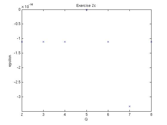
Wow! Already at two integration
points we are at machine precision! Due to the unforseen fact that GLL
differentiation followed by integration will allways yield the exact
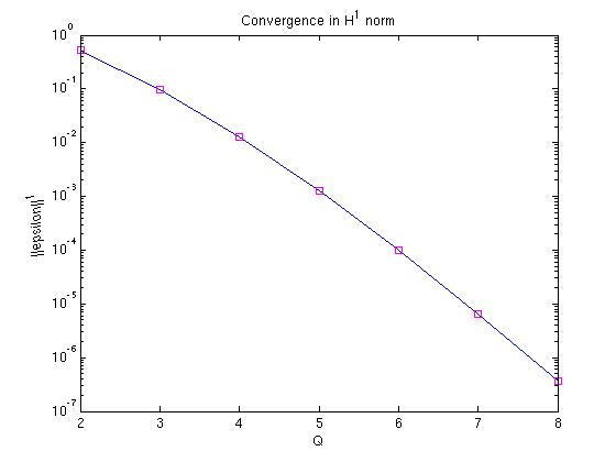
solution we didn't get to see a nice convergence plot. If we however
take the H1-norm of the error, defined as

where l is the length of the
domain, df/dx is the numerically differentiated cosine and df_ex/dx
is the analytically differentiated cosine (thus a negative sine) we do
get a nice plot shown below.