We are now finished with the projection
problem, so we can start solving our first differential equation. The
equation will be the 1-D Helmholtz equation: u_xx - lambda*u(x) =
f(x) (where underscore xx means the second derivative
with respect to x). There won't be any more totally new
concepts but a few changes have to be made to our old codes. I did this
exercise in two parts, the first part will be the making of a
single-element solver and the second part will be a multi-element one.
Because of the similarity with exercises 3 and 4 I called my codes
Helmholtz3.cpp and Helmholtz4.cpp.
To state the problem in the appropriate form we must first write it in the weak form. This is not difficult but attention must be paid to the signs of the different terms. After lifting of the solution my weak form looked like this:
To state the problem in the appropriate form we must first write it in the weak form. This is not difficult but attention must be paid to the signs of the different terms. After lifting of the solution my weak form looked like this:
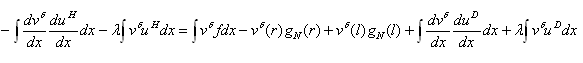
Where the arguments r
and l
mean the right and left boundary respectively (the Neumann bc's are of
course only valid if they are posed as actual bc's). We have to make a
variable which specifies if at a boundary the bc specified in the
variable
Now we will start the final part of the exercises, coding a multi-element-1-D-Helmholtz-solver! Basically no new concepts are needed for this exercise, but still it will not be easy to get your code running. I started with the code of exercise 4b. An important change has to be made to the mapping matrix because the entries of course depend on the bc's posed. A lot of other changes will be necessary but it's mostly coding of what you already understand. My code is only suitable for more than one element (so
bc is a Dirichlet bc or a Neumann bc. Herefor I
made the two-element vector Dirichlet, where the case Dirichlet[0]=1
means that at the left boundary a Dirichlet bc is specified, the case Dirichlet[0]=0
means that at the left boundary a Neumann bc is specified and similar
meanings for Dirichlet[1] at the right boundary. An
important addition to the code
of exercise 3e (which I used as basis) is the differentiation
function diff, which mainly will fill the new vectors dphi1
and dphi2 for construction of the Laplacian matrix L.
Don't forget to define the differentiation matrices D and
Dt. As forcing function I used f(x) = -(pi^2 +
lambda)*sin(pi*x), because the solution u(x) will
(when lambda = 1) then be u(x) = sin(pi*x). It
might be a bit confusing that withevery change of type of bc's the size
of the matrix (Mdim) changes but you'll get used to it.
After a lot of struggles I finally had my code
running, so if this is the case with you too at least you're not the
only one!Now we will start the final part of the exercises, coding a multi-element-1-D-Helmholtz-solver! Basically no new concepts are needed for this exercise, but still it will not be easy to get your code running. I started with the code of exercise 4b. An important change has to be made to the mapping matrix because the entries of course depend on the bc's posed. A lot of other changes will be necessary but it's mostly coding of what you already understand. My code is only suitable for more than one element (so
Nel > 1). This exercise will
demand a
lot of determination but if you succeed you can get yourself a
well-deserved cup
of tea!