Exercise 1

Exercise 1 consists of the coding and testing of a numerical integration (quadrature) program. Part (a) concerns integration of a polynomial over the 1-D standard element [-1,1]. My code for exercise 1a can be found here. I did this via the definition of four functions. The first is called dvector, it allocates memory space so that the pointer which uses this function can be a vector of double precision elements with the length of the argument of dvector. Thus the line:       

    z = dvector(3);

allocates enough memory to the pointer z to be a vector of three double precision elements, the first being z[0] and the last z[2]. The second function I use is the zwgll function which is explained in the compilation and polylib section. After applying this function the pointers/vectors z and w will be filled with the np integration points and weights. Now it is time to specify the function which has to be integrated. For this I made a function called func which fills the double precision pointer p with the values of ksi^6 at the np integration points. By the way, in my codes, functions which fill pointers/vectors are defined as void pointerfunctions, so for example the declaration of func looks like this:

    void *func(int np, double *z, double *p);

These void functions only change the values at the adresses at which their (pointer)arguments point, so a return statement is not necessary. This is different in the fourth function I used which is called integr. This is a double precision function which has got a return statement. It returns the value of the integration! When using this type of function the statement:

    integr(np, w, p);

will thus be interpreted as the value of the integration. In this case it will be the integration of p using np points and weights w.

For part (b), the integration of a polynomial over a non-standard interval, a couple of additions have to be included in the code (which can be found here). Because a mapping function has to be defined we need three extra variables. First a vector is needed to contain the x-coordinate, this is, as usual, done via a double precision pointer x (from now on every variable will be of double precision by default, it will be mentioned when this is not the case). Then we need the Jacobian of the mapping which is defined as a one element vector Jac. The two-element vector bound will contain the boundaries of the integration domain, the left boundary will be bound[0] and the right boundary will be bound[1]. In my code(s) the boundaries are double precision, so to prevent any problems it is best to state them in decimal form. Of these extra variables Jac and x will be determined in the mapping function chi and bound can be given any desired values. Equation (2.31) of chapter 2 of the book specifies the mapping chi and this is just what the function chi does (and of course calculating the Jacobian).

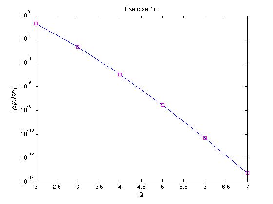
When part (a) and part (b) are completed succesfully part (c) should not be a big problem. Here is my solution. It has only minor changes in comparison with part (b). The changes are the domain, (in the bound vector) which is now [0,pi/2] and the function in func, which now is a sine function. Don't forget to include math.h and remember that pi can be collected by the macro M_PI. Underneath my plot can be seen of the absolute value of the error epsilon on the (logarithmically scaled) vertical axis versus the number of GLL integration points Q. As expected (and explained in exercise 1c) the line is approximately straight.